Rocscience | Mapping Functions: The Newest Addition to Generalized Anisotropic Featured

The Generalized Anisotropic strength type in Slide2 and Slide3 is the most flexible way to model anisotropic materials. Everything is in the user’s hands.

Anisotropy Definition

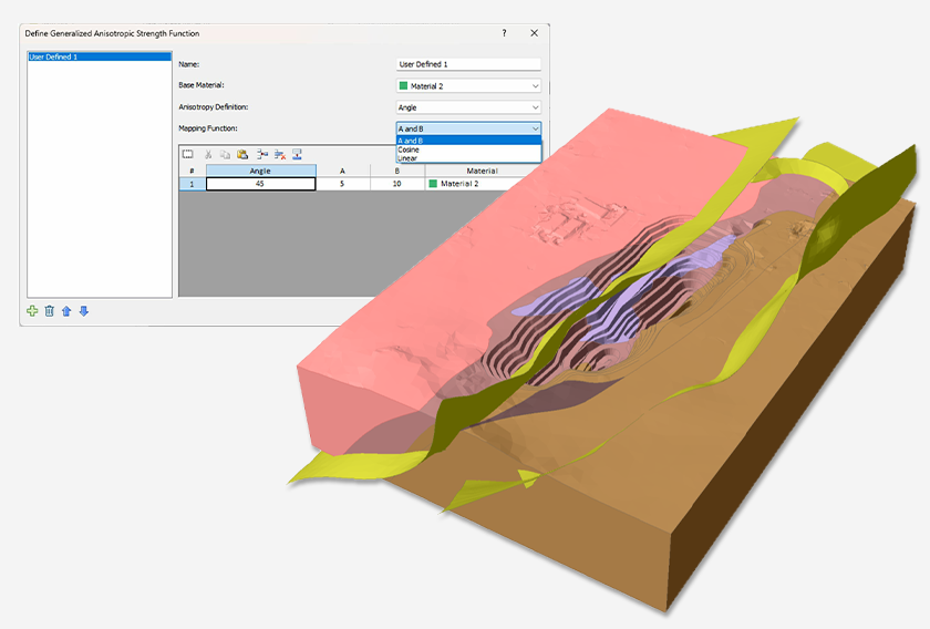
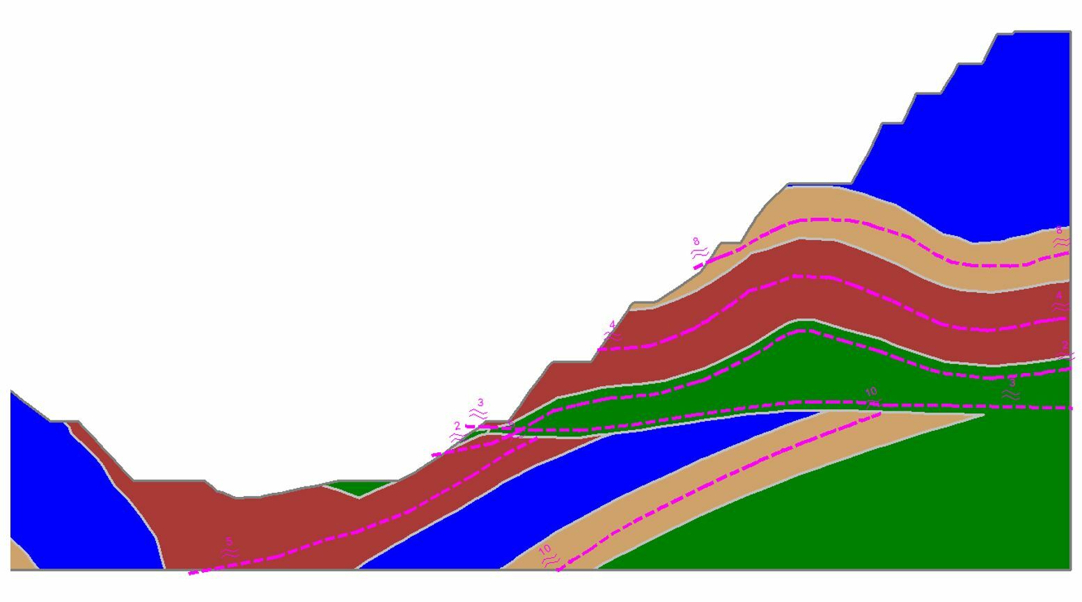
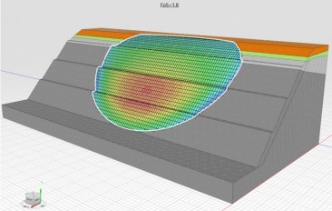
You can specify the direction of anisotropy either using an angle (dip and dip direction in 3D), or an anisotropic surface. While the angle is self-explanatory, the surface allows you to define anisotropy along bedded materials, as shown in Figure 1.

Depending on the direction of sliding, the material will have a shear strength corresponding to either the base material, the joint material, or an intermediate value between the two. In Slide2 and Slide3, you have the power to control exactly how the material strength is calculated from and between these two values.

The A and B Angles

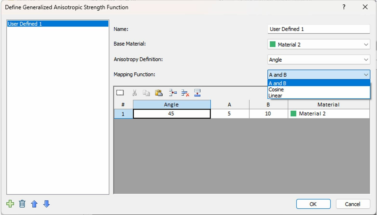
With the A and B angles, you can define how closely aligned the sliding direction needs to be with the joint direction(s) for the strength of the joint material(s) to be considered. Say you have a joint defined in Slide2 at an angle of 45o, with A=5°, and B=10°. This means that the strength of the joint material will be used when the angle of slice base lies in the 45o ± A range (i.e., 40o to 50o), while the strength of the rock material will be used when the angle of the slice base lies outside of the 45o ± B range (i.e., smaller than 35o or bigger than 55o). In between (35o – 40o and 50o – 55o) the strengths are interpolated.

Mapping Functions

The new mapping function dropdown will be added to the latest versions of Slide2 (v9.028) and Slide3 (v3.022). This option gives you the ability to select different interpolation methods. The options will be:

• A and B – as discussed above.
• Linear – interpolates the strength linearly based on the difference between the angle of the slice base and the angle of the joint (i.e. the angle offset). If the angle offset is zero, then the joint material is adopted, whereas if the angle offset is 90° (perpendicular to the joint direction), then the base material is adopted.
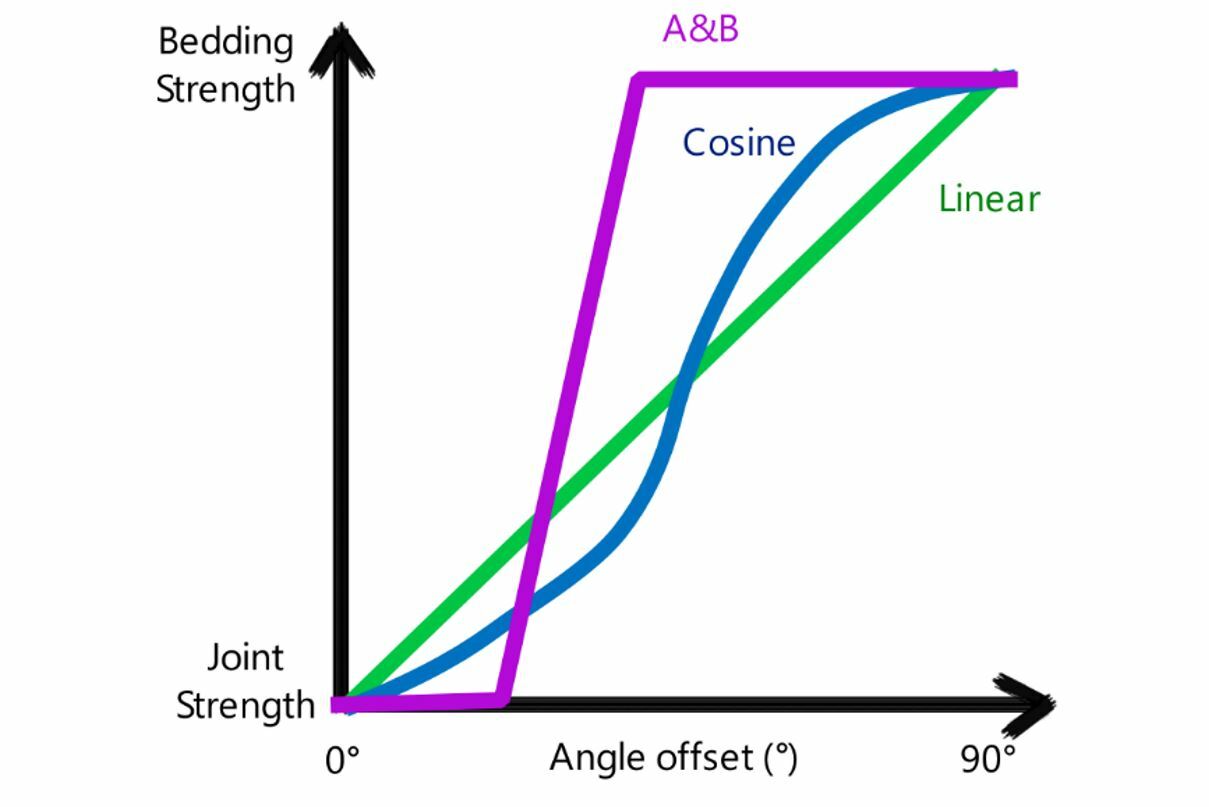
• Cosine – interpolates the strength based on the cosine of the angle offset. If the cosine of the angle offset is 1, then the base strength is used. If the cosine of the angle offset is 0, then the joint strength is used.

A figure showing the interpolation schemes associated with the available mapping functions is shown below.

Slide3-Slide2 Generalized Anisotropic Integration

When exporting your anisotropy from Slide3 to Slide2, it is important that the anisotropy be detectable in the 2D section. In the case of a narrow range for the values A and B, for example, that are smaller than the angle range between the dip direction of the 2D section and the dip direction of anisotropy, the 2D section won’t be able to detect the anisotropy at all. When using the anisotropic integration, a more inclusive mapping function is recommended such as Cosine or Linear.

Why was this option added?

As there are many varying assumptions about the shear strength in anisotropic materials you may wish to employ, this option is another step towards making the Generalized Anisotropic strength type as flexible as possible.