Effect of Joint Orientation on Inter Ramp Stability Sponsored

Anisotropy is an important factor in controlling the stability of rock slopes because it affects the mechanical behavior of the rock mass. Rock masses can have different mechanical properties depending on the orientation of the rock units and the orientation of discontinuities, such as fractures and joints. When the orientation of the discontinuities and the orientation of the rock mass relative to the slope are unfavorable, the rock mass may be more prone to failure, making the slope less stable. Therefore, understanding the anisotropy of a rock mass is crucial for assessing its stability and designing safe slopes. The objective of this example is to demonstrate how GeoStudio can be used to explore the effect of joint orientation on the calculated factor of safety for an inter ramp stability. Specifically, a comparison between 2D and 3D analyses is conducted to evaluate the effect of increased joint obliquity on stability. For a 2D analysis, the only option to account for joint orientation is to calculate an apparent dip. The 3D analysis, in contrast, readily considers the orientation of the anisotropy relative to the slope angle.

Background

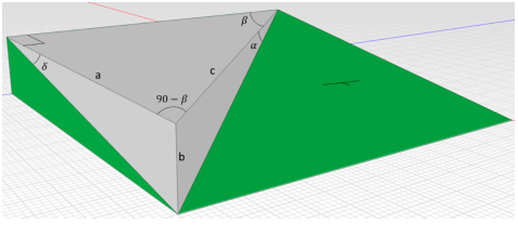
Dip and dip direction are measurement conventions used to describe the orientation of a planar geological feature. The dip is the steepest angle of descent of a tilted feature relative to a horizontal plane (𝛿 in Figure 1). The dip direction is the azimuth (i.e., compass direction) of the dip line; that is, the azimuth of the imagined line inclined downslope. A 2D analysis is ideally aligned with the dip direction of the structures, however, this is often not the case because of the topography. Figure 1 shows a planar feature such as a joint within a rock mass. The vertical plane comprising lines 𝑐 and 𝑏, which is misaligned with the dip direction, is assumed to represent a 2D cross-section. The apparent dip 𝛼 can be calculated as:

α = tan^-1(sin β tan δ)       Equation 1

β = γ − θ         Equation 2

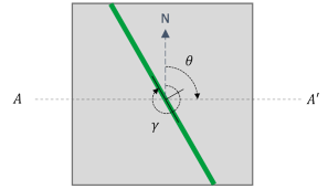
where 𝛿 is the true dip measured along the maximum slope direction of the structure (Figure 1) and 𝛽 is the angle between the strike direction of the planar feature (𝛾) and the bearing of the cross-section (𝜃), as shown Figure 2.

Numerical Simulation

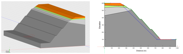
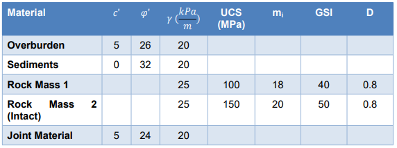
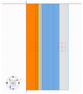
Figure 3 presents the geometry and geology of the analysis domain. The slope face has an Eastward bearing. The geology comprises overburden soil (orange), sediments (green), and 2 rock units (light/dark grey). Joints, or weak layers, are assumed ubiquitous in Rock Mass 2, which is the lowermost unit. Table 1 presents the inputs for the strength models. The strength of the overburden and sediment layers were described by a Mohr-Coulomb model, while the intact rock masses were characterized as Hoek-Brown materials. The Hoek-Brown materials were created by entering the Uniaxial Compressive Strength (UCS), intact rock parameter (mi), Geological Strength Index (GSI), and the disturbance factor (D). The strength of the joints in Rock Mass 2 were defined by a Mohr-Coulomb material model with a cohesion and friction angle of 5 kPa and 24°, respectively.

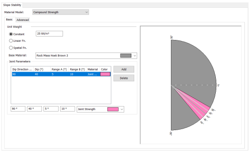
Rock Mass 2 requires special consideration since a joint set is present. The Compound Strength model accounts for anisotropic (i.e., directionally dependent) strength caused by the presence of planar structures within a soil/rock matrix. The Compound Strength model composes a Base Material and Joint Parameters (Figure 4). In this example, Rock Mass 2 (Intact) is the Base Material and there is a single joint set dipping at 40°, with its strength defined by the Joint Material (Table 2). The A and B angles of 5° and 10°, respectively, control the transition of the strength from the joint material to the intact rock strength. Four cases are considered in the associated project file, with the dip direction of the joint set to 90° (i.e., East), 80°, 70°, and 60°, which corresponds to a strike 𝛾 of 360° (0°), 350°, 340°, and 330° (Figure 5).

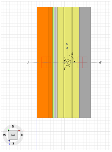
The 2D analyses are completed on Section A-A’ (Figure 5), which has a bearing 𝜃 = 90° (Figure 5). Equation 1 and Equation 2 can be used to calculate the apparent dip for all four scenarios. The results are summarized in Table 2.

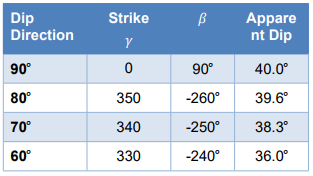
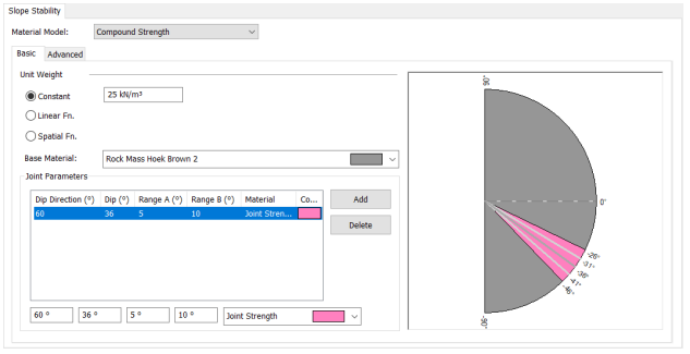
Figure 6 presents Compound Strength model defined for a 2D analysis with the dip direction of 60°. In 2D, the solver resets the dip direction to 90° (i.e., East) if the user entered value is between 0° and 180°, and to 270° if ≥ 180°. Hence, the apparent dip (36°; Table 2) is specified when the bearing of the 2D cross-section is oblique to the true dip direction.

There are two geometries in the GeoStudio project: one for the 2D analysis branch and one for the 3D analysis branch (Figure 7). The 3D geometry was created by importing the 2D analysis (Figure 8), which automatically extrudes the section one unit in the z-direction. The extrusion distance was changed to 2000 m by right-clicking and editing the Extrude operation in the Design History.

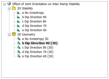
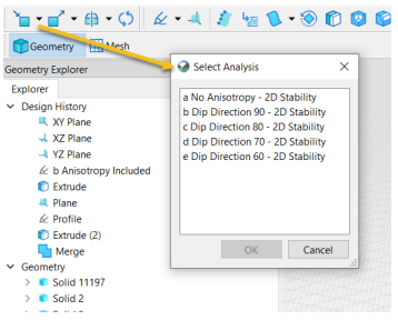
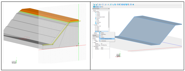
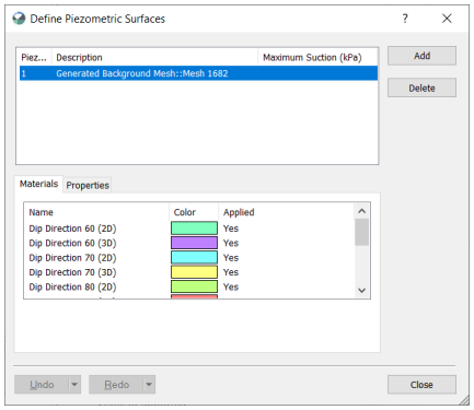
There are five analyses under each geometry, including one for the base case (no anisotropy) and four to model the various joint orientations. The pore-water pressure conditions were defined using a piezometric surface (Figure 3). In 3D, the piezometric surface was created by sketching the corresponding line on the XY Plane, extruding it across the length of the domain, and then converting the surface to a background mesh (Figure 9). Once done, the background mesh is available under the Define | Piezometric surfaces dialogue box when selecting ‘Add’ (Figure 10).

The entry-exit slip search technique was used in both the 2D and 3D analyses. The definition was selected to ensure that a deep-seated mode of failure was analyzed (i.e., inter-ramp stability). The entry/exit grid in 3D is centered on the domain and extends 100 m in both directions off center (Figure 11). Two increments along both sides of the grid reduce the number of slip surfaces and therefore reduce computational time. An ellipsoidal slip surface shape was selected for 3D. Ellipsoids are generated by calculating the principal semi-axis 𝑐 = 𝑘𝑎, where 𝑘 is the aspect ratio, with aspect ratios of 0.8, 1.0, and 1.2. A value of 1.0 produces a sphere, while 0.8 and 1.2 produce an ellipsoid that is shorter and longer in the direction orthogonal to the principal axis, respectively.

Results and Discussion

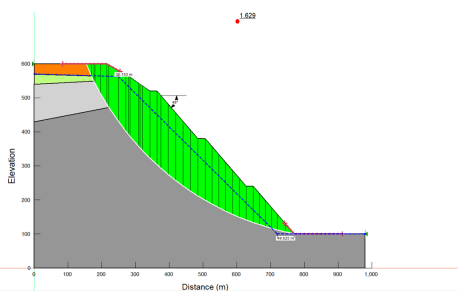
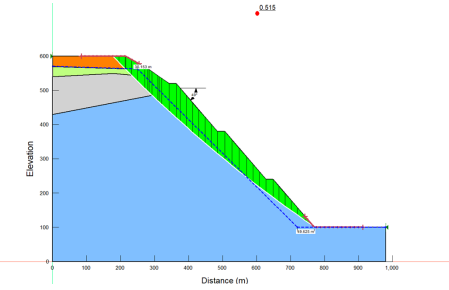
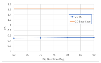
Figure 12 and Figure 13 present the 2D results for the base case (without anisotropy) and the case where the joint set has a dip direction of 90. Figure 14 summarizes the 2D factors of safety (F.S.) for all cases. The factor of safety decreases from about 1.63 to 0.52 when the joint set is aligned with sliding direction (i.e., East). The anisotropy feature has a friction angle of 24 while the overall slope angle is greater than 4o, so naturally the anisotropy will govern the stability. The shape of the slip surface, which is planar, confirms this supposition. Figure 14 demonstrates that the F.S. is essentially unchanged when the dip direction of the joint set is oblique to the East facing slope. As shown in Table 2, the apparent dip decreases only marginally over the range of dip directions. Moreover, the smaller apparent dip angles cause the joints to daylight further up the slope, causing the F.S. to drop slightly from 0.52 to 0.50 at a dip direction of 60

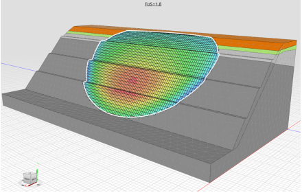
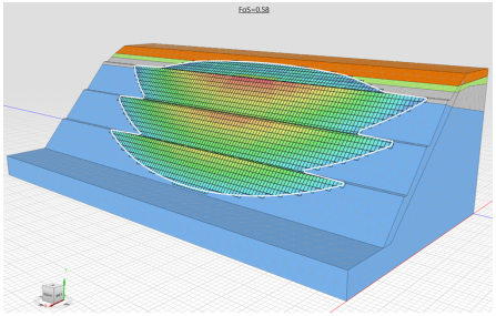
The results of the 3D analyses provide a different understanding of the role of the joint sets. Figure 15 and Figure 16 present the 3D results for the base case and the case where the joint set has a dip direction of 90. Figure 17 summarizes the 3D F.S. for all cases. The factor of safety decreases from about 1.8 to 0.6 with the introduction of Eastward dipping joints, which is like the 2D case. The factor of safety for 3D cases with no anisotropy and a dip direction of 90 is about 10% higher than the 2D equivalents due to the ‘end effect’, where the slip surface reduces in size along its perimeter.

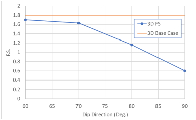
In 3D, the F.S. increases substantially as the dip direction of the joint set becomes oblique to the bearing of the slope face (Figure 17). Unlike the 2D scenarios, the increased obliquity results in less of the slip surface aligning with the anisotropy. Figure 18 presents the friction angle at the column bases versus z-coordinate for dip directions of 90° and 60°. Each series corresponds to a row of columns with the same x-coordinate. A significant number of columns have the lower friction angle (24°) of the joint set when the joints dip in the direction of the slope face (i.e., 90°). In contrast, far less columns have a lower friction angle when the dip direction of the joint set is oblique to the slope face. Both graphs reflect the transition from the joint set to intact rock mass, as characterized by the A and B range in Figure 4.

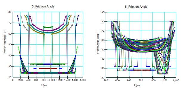
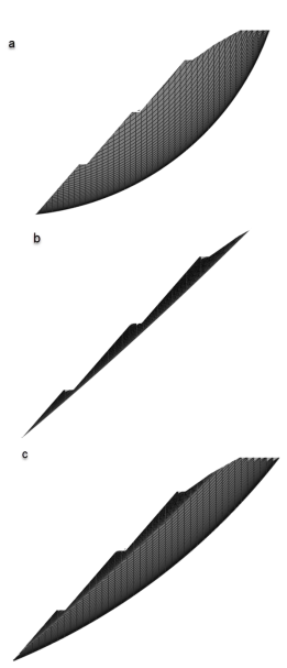
Figure 19 presents profiles of the 3D slip surfaces for the base case and dip directions of 90°and 60°. For the base case, the critical slip surface is deep (a). The introduction of anisotropy results in a very shallow slip surface given that the dip of the anisotropy is essentially equal to the overall slope angle (b). The increased obliquity means that the critical slip surface must increase its driving mass to overcome the increased strength from the intact rock (c).

Summary

The effect of rock anisotropy on the inter ramp stability of an open pit mine is significant. This example demonstrates that a 2D analysis fails to capture the effect joint orientation on the calculated F.S. The obliquity of the joint set relative to the cross-section orientation can only be captured via the apparent dip in a 2D analysis. The apparent dip decreases relative to the true dip as the obliquity increases. In this example, the joint sets changed from being nearly parallel with the slope to being a few degrees shallower than the slope face. The overall effect on the factor of safety was marginal because most of the critical slip surfaces were aligned with the joint set.

In contrast, the effect of obliquity on the 3D F.S. was significant because less of the slip surface was aligned with the anisotropy as the obliquity increased, despite the Compound Strength model having a wide range of base angles to transition from the anisotropy to the intact rock strength. Finally, it should be noted that the analyses presented herein are intended to demonstrate specific functionality in SLOPE3D. A more comprehensive study of the effect of obliquity should include wedge-like slip surfaces and optimization of the slip surface shape.