Dewatering example on a specific deep well system with GeoStudio Sponsored

The objective of dewatering is to lower the groundwater table to prevent significant groundwater flow into an excavation, and/or to ensure slope stability. The preferred dewatering system will depend on hydrogeological conditions and construction requirements. In the case of slopes and excavations, the groundwater table can be lowered using a combination of methods, such as deep wells, wellpoints, vacuum wells, and horizontal wells. Deep well systems are often used for dewatering slopes and excavations when large drawdowns are required. This type of system generally consists of an array of pumping wells located near the excavation or slope. The combined effect of the array lowers the groundwater table over a wide area. The active pumping system must be set below the groundwater table whereas the bottom of the wells must be set deep enough to allow flow without excessive head loss.The objective of this example is to illustrate how to model deep well systems in three-dimensional environments, and to verify the water-flow formulation against a well-known benchmark. To do so, the example will discuss a specific deep well system, and provide insight into an approach formodeling pumping wells.
Numerical Simulation
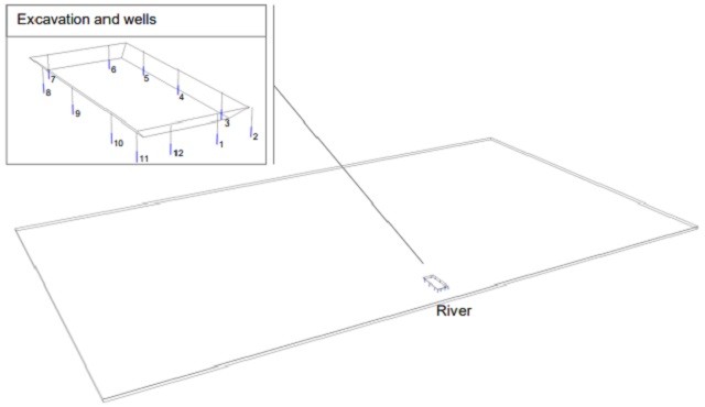
The deep well system, taken from Mansur and Kaufman’s (1962) chapter on dewatering, consists of a large, 770 foot-long by 370 foot-wide, 40 foot-deep excavation in a 90 foot-deep unconfined / sandy aquifer. In order to capture the full effect of the river, the domain was extended 10,000 feet beyond the excavation in each direction. As shown in Figure 1, the centerline of the excavation is located 1000 feet from the edge of the river. The dewatering system consists of twelve pumping wells, located 5 feet from the crown of the excavation slope. The wells are provided with 40 feet of 10-inch diameter screens, and the pumping rate at each well is assumed equal to 1150 gpm (or 2.56 ft³/sec).
The Saturated/Unsaturated Material Model was used to describe the sandy aquifer. Although optional in steady-state analyses, the volumetric water content function was used to estimate the hydraulic conductivity function. The volumetric water content function was taken as that of a typical sand with a porosity of 0.35 and a soil-structure compressibility of 5×10⁻⁸ /psf. The saturated hydraulic conductivity was set equal to 3.33 x 103 ft/s.
The river level was assumed to remain constant, at 85 feet of elevation, and a potential seepage face was assumed to prevail on the inner surfaces of the excavation. Although the pumping wells can be modeled as three-dimensional cylindrical objects, this can create numerical difficulties in large-scale problems. These difficulties can be alleviated by representing the wells as lines with prescribed water flux and surface perimeter. In this study, each pumping well was modeled as a line representing the effective screen length. The effective screen length accounts for head loss in the wells and was determined by numerical experimentation. The water flux along the effective screen length was computed as where is the surface perimeter and is the 𝑄𝑝𝑢𝑚𝑝𝑖𝑛𝑔 (𝑃𝐿𝑒 ) 𝑃 𝐿𝑒 effective screen length. The downside to this approach is that high hydraulic gradients may prevail near the lines where pumping occurs. To mitigate this issue, the element edge length was set equal to one foot, and mesh refinement distance was set to ten feet along the effective screen length. In this example, the finite element mesh was generated with 200 ft edge lengths in a tetrahedral pattern, which resulted in 56105 nodes and 191796 solid elements.
Results and Discussion
Figure 2 shows the total head isosurfaces and phreatic surface from two different perspectives. As expected, the array of pumping wells prevents groundwater flow from entering the excavation, and results in lowering of the total head and phreatic surface beneath the excavation. The total head is also found to be highest in the portion of the excavation closest to the river. Overall, the deep well system lowers the phreatic surface, and in so doing, provides additional stability to the side slopes and base of the excavation.
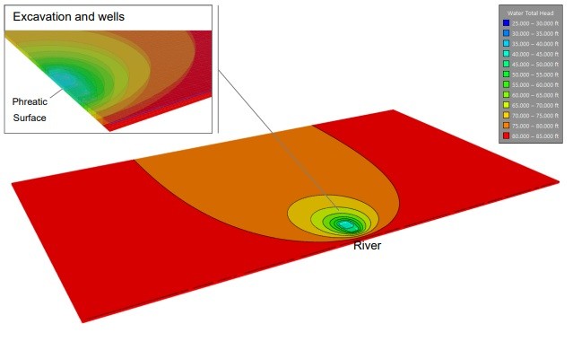
Figure 3 shows the total head beneath the center of the excavation, and reveals that it is essentially constant at 44.86 ft.
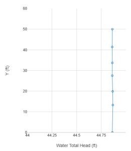
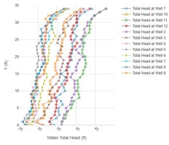
Figure 4 shows the total head along the length of the different wells. As in reality, the pumping process results in nearly constant values of total head along the screened portion of the wells. For instance, the total head along the effective screen length of well number four remains approximately constant at 31.04 ft. The total head is highest in the wells located nearest to the river, at both the west and east edges of the excavation (wells two and eleven). The distribution also appears near symmetrical about the axis perpendicular to the river.
Adequacy of these results can be assessed by comparing them to those obtained using the method of images. As reported by Mansur and Kaufman (1962), the method of images results in values of total head of 44.5 and 32 feet beneath the center of the excavation and at well number four, respectively. These results show good agreement with the model predictions. It's worth noting that inadequate mesh constraints around the wells can introduce significant errors in the computed total head values near those locations. This sensitivity can be quickly assessed by adjusting the element edge length and/or the mesh refinement distance around the effective screen length of the wells.
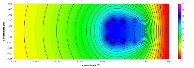
Figure 5 presents a plan view contour plot of drawdown, a visualization commonly favored by hydrogeologists for its clarity and efficiency in interpreting changes in total head. This type of plot offers a quick and intuitive understanding of groundwater flow patterns and the influence of pumping wells within the excavation area. These drawdown contours were generated using the GeoStudio scripting API, leveraging the script available through the Learning Management System. This streamlined workflow allows users to produce high-quality visualizations with minimal effort, ensuring consistency across analyses and facilitating rapid interpretation of model results.
Summary and Conclusions
The capabilities of the software were assessed with a benchmark problem for deep well systems in three-dimensional environments. The results were shown to capture the general trend of the groundwater flow system, and to be in close agreement with those provided by the method of images. Though it was shown that pumping wells could be modeled as lines with prescribed water flux and surface perimeter, it was found that mesh constraints had to be applied around the screened portion of the wells for the sake of accuracy.
Sources: GeoStudio - SEEP3D - Dewatering - Deep Well Systems - Information [PDF], GeoStudio - SEEP3D - Dewatering - Deep Well Systems - Project [gsz]
Want to read more like this story?

Beacon Hill Station Dewatering Project
Aug, 21, 2024 | NewsDewatering wells effectively lowered groundwater levels up to 60 ft before excavation of the shaft...

Bear Creek Dam Dewatering and Excavation Support Project
Aug, 14, 2024 | NewsKeller performed construction dewatering and excavation support during the Bear Creek Dam remediati...

Gregg Drilling & Testing Water Well Services
Sep, 07, 2016 | NewsWith over 30 years experience drilling in California and surrounding states, Gregg Drilling can hand...

Brigantine Connector Project
Oct, 07, 2024 | NewsDuring the construction of the 2,900-ft-long tunnel/depressed roadway section of the Atlantic City-...

3D Finite Element Analysis of a Deep Excavation & Ground Response Evaluation
Jun, 13, 2022 | NewsSignificant ground movements due to deep surface excavations can seriously impact neighbouring infr...

Crane Valley Dam dewatering system design project
Jun, 19, 2024 | NewsKeller North America worked closely with the geotechnical engineer to design a dewatering system ca...

Dewatering and earth retention solutions at Atlantic Park Surf
Nov, 12, 2025 | NewsKeller provides dewatering and earth retention solutions at a new wave park, located just two block...

UK’s first deep geothermal energy plant in 37 years begins operations
Jun, 19, 2023 | NewsEden project’s deep geothermal heating plant, located in Cornwall, began operations on Monday, June...

Deep Supported Excavation in Urban Environment
May, 09, 2019 | Education"Measured vs. Predicted behavior", Degree thesis of Dimitris P. Zekkos, Civil Engineering Departmen...
Form
Looking for more information? Fill in the form and we will contact Seequent, The Bentley Subsurface Company for you.
On This Day
July 12th 1945
READ MORE
Related Video

Trending
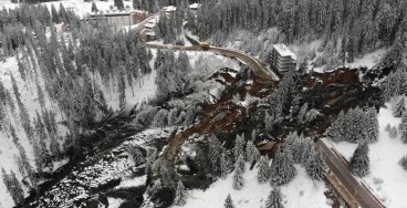
Active landslide threatens long-term connectivity in southern Bulgaria


PLAXIS example: Westergaard's added mass for hydrodynamic pressures

Rock Mass Classification Systems: A Global Review of Use and Dominant Approaches
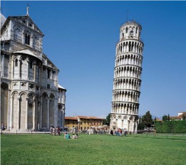
How does the Leaning Tower of Pisa survive earthquakes
Emergency ground stabilisation protects rail works near Salford Central