Landfill Gas Monitoring Systems
Contents [show]
Introduction
Landfill gas emissions can cause serious problems that are now widely known, especially when the gases, after escaping from the site, accumulate in enclosed spaces where they can present a latent hazard, giving rise to explosions under the certain conditions. Landfill gas monitoring is therefore a critical concern for landfill operators and has become part of the legal requirements for the design, operation, and closure.
Landfill gas, which has approximately 50 percent methane and 50 percent carbon dioxide with trace components, is produced through bacterial decomposition, volatilization and chemical reactions. In addition, a number of factors influence the quantity of gas that a MSW landfill generates and the components of that gas. However, adverse environmental effects of landfill gas are increasingly being felt today. In order to reduce risk from landfill gas hazards, engineers generally use two methods to quantify gas emissions from landfill: they either estimate the emissions or measure them. The former is landfill gas modeling while the latter is landfill gas monitoring.
The goal of landfill gas monitoring is to detect the presence of gas, and to predict the quantity of gas as well as location in which to expect high gas concentrations. In this context, there are lots of landfill gas monitoring methods. These methods vary for different landfills. To choose proper monitoring methods, many factors should be considered, such as landfill types, site conditions, regulatory requirements, costs, but most importantly, the objective of monitoring, or the parameters to be monitored.
Generally, all gas monitoring activities can be classified into five categories:
- Soil gas monitoring (Subsurface monitoring)
- Near surface gas monitoring
- Emissions monitoring
- Ambient air monitoring
- Indoor air monitoring
There are too many monitoring techniques of each category to discuss all of them in detail in this report. Also, there are “intersections” in these monitoring activities, for example, emissions monitoring, can be a surface monitoring or a subsurface monitoring, and the monitoring parameters and techniques for ambient air and indoor air are very similar.
Emissions monitoring focuses on the measurement of gas emission rate; flux chambers are usually used for emissions monitoring. Surface monitoring and subsurface monitoring focus on the concentration of landfill gas, such as methane.
In this report, soil gas monitoring is discussed in detail, including installation and sampling methods. And one or two techniques for near surface monitoring and emissions monitoring are introduced.
Finally, the Landfill Gas Monitoring Regulations are introduced at the end. It includes how to determine if a landfill gas need to be monitored, and guidelines or requirements for gas collection system, gas control device, and compliance schedule, and device removal.
Landfill Gas
The following sections provides background information about landfill gas: what it is composed of, how it is produced, why landfill gas monitoring is important, and the conditions that affect its production. It also provides information about how landfill gas moves and travels away from the landfill site. Finally, the sections present an overview of the landfill gas modeling that might be applied to estimate landfill gas composition.
Landfill Gas Overview
LFG (landfill gas) is a natural byproduct of the decomposition of organic material in anaerobic (without oxygen) conditions. Landfills are the second largest human-caused source of methane in the United States, accounting for approximately 18.2 percent of U.S. methane emissions in 2013 (EPA gas portion). Methane is a potent greenhouse (heat trapping) gas with a global warming potential that is 25 times greater than carbon dioxide (EPA, 2015a). One million tons of MSW produces roughly 432,000 cubic feet per day (cfd) of LFG and continues to produce LFG for as many as 20 to 30 years after it has been landfilled. With a heating value of about 500 British thermal units (Btu) per standard cubic foot, LFG is a good source of useful energy, normally through the operation of engines or turbines. Some landfills collect and use LFG voluntarily to take advantage of this renewable energy resource while also reducing GHG emissions. However, its adverse effects to humans as well as environments are also significant today.

Figure 1. Landfill gas (Diagram from Gazasia)
Types and Amounts of Compounds of Landfill Gas
Landfill gas is composed of a mixture of hundreds of different gases. By volume, landfill gas typically contains: 45% to 60% methane (CH4) and 40% to 55% carbon dioxide (CO2). Landfill gas also includes small amounts of nitrogen, oxygen, ammonia, sulfides, hydrogen, carbon monoxide, and non-methane organic compounds (NMOCs) such as trichloroethylene, benzene, and vinyl chloride. Specifically, Table 1 represents the gas composition of the Fresh Kills municipal solid waste landfill in USA (Bart et al., 1998). The example shows typical characterization of the composition of the landfill gas and the variability in the gas composition from 250 separate landfill gas samples.

Figure 2. Typical constituents found in municipal solid waste landfill gas; Trace constituents are benzene, toluene, vinyl chloride, trichloroethylene, dichloromethane etc. (G. Tchobanoglous et al, 1993)

Figure 3. Typical concentrations of some trace compounds found in landfill gas (G. Tchobanoglous et al, 1993)
Table 1. Average landfill gas composition, unit: parts per million by volume (Bart et al., 1998)

Concerns Caused by Landfill Gas
There are several concerns with landfill gas (USACE, 1995):
- Methane gas is highly combustible, making it potential hazard in the landfill environment or in structures on adjacent properties.
- Landfill gas is capable of migrating significant distances through soil, thereby increasing the risk of explosion and exposure. Serious accidents resulting in injury, loss of life, and extensive property damage may occur where landfill conditions favor gas migration.
- As landfill gas is produced, the pressure gradient upward may create cracks and disrupt the geomembrane in the landfill cover.
- Methane gas is an asphyxiant to humans and animals in high concentrations.
- Migrating gas may cause adverse effects such as stress to vegetation, by lowering the oxygen content of soil gas available in the root zone.
- Gas generated at landfills and vented to the atmosphere frequently emits bad odors, causing annoyance to people residing nearby.
- Emissions of NMOCs in landfill gas may be contributing to the degradation of local air quality. Vinyl chloride from landfills has been found to be present in substantial concentrations in landfill gases, presenting health and safety concerns.
- Methane gas, a “greenhouse gas,” contributes to the possibility of global warming of Earth’s climate.
- Uncontrolled landfill gas is a loss of potential resources; instead, it can be a satisfactory fuel for a wide variety of applications.
Table 2. Examples of landfill gas hazards (Gino Yekta, 2014)

Landfill Gas Generation
Approximately 251 million tons of MSW were generated in the United States in 2012, with about 54 percent of that deposited in landfills (EPA, 2015b). Landfill gas is generated by the natural process of bacterial decomposition of organic material contained in landfills. A number of factors influence the quantity of gas that a MSW landfill generates and the components of that gas. Among them, there are certain processes that form landfill gas including bacterial decomposition, chemical reactions, and volatilization (Gino Yekta, 2014).
- During bacterial decomposition, organic waste (which includes food waste, green waste, wood and other paper products) is broken down by bacteria naturally present in the waste and in the soil that is used to cover the landfill. Bacteria decompose organic waste in five distinct phases and changing gas composition during each phase.
- During chemical reactions, Non-Methane Organic Compounds (NMOCs) are created,
- During volatilization, landfill gases can be created when certain wastes, particularly organic compounds, change from a liquid or a solid into a vapor.
- Bacterial decomposition has four phases as shown in Figure 4. The composition of the gas produced changes with each of the four phases of decomposition. Landfills often accept waste over a 20 to 30 year period, so waste in a landfill may be undergoing several phases of decomposition at once. This means that older waste in one area might be in a different phase of decomposition than more recently buried waste in another area.

Figure 4. Production phase of typical landfill gas (ATSDR, 2001)
Phase I: Aerobic bacteria which live only in the presence of oxygen consume oxygen while breaking down the long molecular chains of complex carbohydrates, proteins, and lipids that comprise organic waste. The primary byproduct of this process is carbon dioxide. This phase could last for days or months, depending on how much oxygen is present. Phase I continues until available oxygen is depleted.
Phase II: Phase II is an anaerobic process which does not require oxygen. In this phase, bacteria convert compounds created by aerobic bacteria into acetic, lactic and formic acids and alcohols such as methanol and ethanol. The landfill becomes highly acidic. As the acids mix with the moisture present in the landfill and nitrogen is consumed, carbon dioxide and hydrogen are produced.
Phase III: Anaerobic bacteria consume the organic acids produced in Phase II and form acetate, an organic acid. This process causes the landfill to become a more neutral environment in which methane-producing bacteria are established by consuming the carbon dioxide and acetate.
Phase IV: The composition and production rates of LFG remain relatively constant. LFG usually contains approximately 50-55% methane by volume, 45-50% carbon dioxide, and 2-5% other gases, such as sulfides. LFG is produced at a stable rate in Phase IV, typically for about 20 years; however, gas will continue to be emitted for 50 or more years after the waste is placed in the landfill.
Gas generation in landfill is affect by the following factors (USACE, 1995):
- Quantity and composition,
- Compaction,
- Age,
- Presence of oxygen in the landfill,
- Moisture content (very important), and
- Temperature
Migration Mechanisms
Once gases are produced under the landfill surface, they generally move away from the landfill. Main factors influencing the migration of landfill gas are (Sharma and Reddy, 2004):
- Molecular effusion
- Diffusion (response to concentration gradient). Moving from high concentration to low concentration in order to be in equilibrium.
- Convection (response to pressure gradient).
Molecular effusion occurs at the surface boundary of the landfill with the atmosphere. When the material has been compacted and has not been covered effusion is the process by which diffused gas releases from the top of the landfill. For dry solids, the principal release mechanism is direct exposure of the waste vapor phase to the ambient atmosphere.
Molecular diffusion occurs in gas systems when a concentration difference exists between two different locations within the gas. The diffusive flow of gas is in the direction in which its concentration decreases. The concentration of a volatile constituent in the landfill gas will almost always be higher than that in the surrounding atmosphere, so the constituent will tend to migrate to a lower concentration area.
Convection is the movement of landfill gas in response to pressure gradients developed within the landfill. Gas will flow from higher to lower pressure regions and from the landfill to the atmosphere. Where it occurs, the convective flow of gas will overwhelm the other two release mechanisms in its ability to release materials into the atmosphere. The rate of gas movement is generally orders of magnitude faster for convection than for diffusion. For most cases of landfill gas, diffusive and convective flows occur in the same direction. The transport mechanisms above are affected by the following factors:
- Permeability,
- Depth of groundwater,
- Condition within the waste,
- Moisture content,
- Human-made features, and
- Landfill daily cover and cap systems.
Landfill gas modeling
Engineers generally use one of two methods to quantify gas emissions from landfill: they either estimate the emissions or measure them (ATSDR, 2001). In order to estimate landfill gas emissions, engineers conduct calculations or use models to predict the rate at which sources may release chemicals to the air. LFG modeling is the practice of predicting gas generation and recovery based on past and future waste disposal histories and estimates of collection system efficiency (EPA, 2015b). It is very important in the project because it provides an estimation of the amount of recoverable LFG that will be generated over time. In addition, LFG estimation is needed in performing risk evaluations, demonstrating compliance with regulatory limits, obtaining permits, and designing emission control systems for solid waste landfills. There are several approaches for predicting and analyzing LFG.
The EPA’s LandGEM (EPA, 2005) is a Microsoft Excel-based software application to calculate estimates for methane and LFG generation. The model uses the first-order decay equation and assumes that methane generation is at its peak shortly after initial waste placement (after a short time lag when anaerobic conditions are established in the landfill). The model also assumes that the rate of landfill methane generation then decreases exponentially (first-order decay) as organic material is consumed by bacteria.

Where:
QCH4= estimated methane generation flow rate (in cubic meters per year or average cfm)
i = 1-year time increment
n = (year of the calculation) – (initial year of waste acceptance)
j = 0.1-year time increment
k = methane generation rate (1/year)
Lo= potential methane generation capacity (m3per Mg or cubic feet per ton)
Mi= mass of solid waste disposed in the ith year (Mg or ton)
Tij= age of the jth section of waste mass disposed in the ith year (decimal years)
Even though LandGEM is the most widely used for LFG modeling and is the industry standard for regulatory as well as non-regulatory applications in the United States, LandGEM may not be appropriate for other countries with significantly different climates or a different landfill waste types. Thus, numerous international LFG models are designed to include adjustments to account for limits to LFG generation and collection caused by conditions at dump sites. Table 3 below represents several models including their assumptions, weak points, and strengths.
Table 3. List of different of LFG prediction model and their specification (revised from Kamalan et al., 2011)

Estimating LFG generation is a critical component of a project assessment and conceptualization because the results are used to estimate the size of the project, project design requirements, expected revenue, and capital and operating costs. However, accurately predicting the total LFG and methane generation can be difficult for many stakeholders because it requires selection and use of an appropriate LFG model among several options, consideration of local conditions that affect LFG generation, and an understanding of the uncertainty inherent with LFG modeling. The value of LFG estimates also heavily depends on the quality of data used in the model; accurate consideration of factors such as annual waste composition, estimated growth rates disposal rates, and the participation of an experienced LFG modeler. The LFG amount also could be estimated by methane generation since methane is big content of Landfill gas. The default methane content of LFG is 50 percent, which is both the industry standard value and LMOP’s recommended default value (EPA, 2015b). Table 4 shows the qualitative comparison of methane generation models by Hans Oonk (2010).
Table 4. Summary of the landfill methane generation models, from ++: very good to --: very poor (Hans Oonk, 2010)

In some cases, engineers will actually measure the gas emissions from landfills. Measuring gas emissions from an entire landfill is a challenging task, primarily because landfill emissions can occur over a surface that spans hundreds, or even thousands, of acres. The landfill gas monitoring is discussed in following sections in detail.
Overview of Landfill Gas Monitoring
3.1 Overview of Landfill Gas Monitoring
In general, monitoring of gases that emanate from landfills falls into the following five categories (Agency for Toxic Substances and Disease Registry, 2001):
- Soil gas monitoring
- Near surface gas monitoring
- Emissions monitoring
- Ambient air monitoring
- Indoor air monitoring
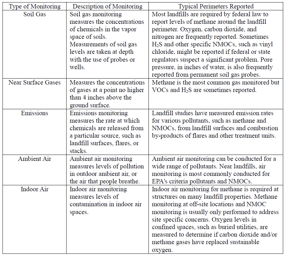
Table 5 presents a brief overview of each type of monitoring. For each type of monitoring activities, there are many gas sampling approaches and monitoring techniques, and unfortunately not all of them can be covered in this report. Some monitoring methods can be used to more than one monitoring activity. However, all the monitoring techniques can be classified from the following four aspects:
- Location of monitors (Subsurface, Surface, and Enclosed Space)
- Portable / Stationary sampling equipment
- Portable monitors: Usually hand-held instrument that can be easily carried around a landfill, which can be used to find the source of methane leaks.
- Stationary monitors: are installed at a fixed location, to monitor gas during a time period. Usually can get higher quality data than portable monitors.
- Grab sampling / Continuous monitoring
- Grab sampling: A one-time measurement at specific location and time.
- Continuous monitoring: Monitoring during a duration of time, through which we can see the changes over a time period.
- Analysis of samples in the laboratory / analysis in the field
- In the lab: expensive but more accurate.
- In the field: more convevient.
Different monitoring methods should be selected for different landfills, considering site conditions, monitoring concerns, financial costs, regulatory requirements and other factors.
Table 5. Types of gas monitoring methods (source: ATSDR, 2001)
Soil Gas Monitoring
3.2 Soil Gas Monitoring
Soil gas monitoring is the measurement of concentrations of gases in the subsurface. Methane is the major landfill gas targeted by soil gas monitoring, because methane is the major cause of landfill explosion and fire incidence.
Soil gas samples are collected using temporary probes or permanent monitoring wells. During sampling, the air pressure and water table in the soil must be known well by the technicians, because this two factors will significantly influence the mitigation of soil gas. Figure 5 shows three different kinds of tips of monitoring probes.


Figure 5. Three kinds of tips (From left to right) (a) Original Gas Vapor Probe Kit, (b) Dedicated GVP Tip, (c) Retract-A-Tip GVP Tip (source: AMS, Inc.)
Nowadays, various soil-gas well designs exist. The main documents dedicated to soil-gas sampling (ASTM D 5314-92; 011, VDI 3865-2; 014, ISO 10381-7; 013) do not precisely define how they should be implemented. (CityChlor, 2013). In the following part, the basic installation procedure of both temporary and permanent soil-gas monitoring wells are introduced, and then some sampling methods which can be used in soil-gas monitoring are discussed.
Temporary soil-gas wells
The installation of temporary soil-gas wells are usually used for perfoming a grab sampling, so it can't be used for long time monitoring or real time tracking of soil gas. Temporary wells, compared with permanent wells, are rapid to set up, which minimize the disturbance to the soil gas. So sampling can be carried out once the wells are installed, we don't need to wait for the "stabilization".
Among the different temporary soil-gas well designs, two main methods are used: rod and direct push systems.
Rod method, as shown in figure 6, firstly a rod is driven into the ground, then a specific casing with screened interval on its bottom is advanced into the borehole. The casing is linked to a specific sampling system (see 3.3). This method is only used for sampling at a shallow depth because of the rod can't be drilled to deep soil.

Figure 6. Rod method (INERIS)
For the direct push method, fistly, drill a borehole using a Percussion Hammer (Figure 7). Then push a rod equipped with a steel tip to the target depth. After that, the rod is withdrawn to expose target interval, through which the soil-gas will be collected by a pump.
Figure 8 shows two kinds of sampling devices. The drive point of the expendable tip samplers is left in the ground. When sampling ends, the whole system is pulled out from the ground and a new drive point is mounted before taking another sample at greater depth or at another location. In contrast, The driving point of retractable probe can be gathered again with sampling tool, so the system don't need to be pull out and can advance to greater depth for another sample.
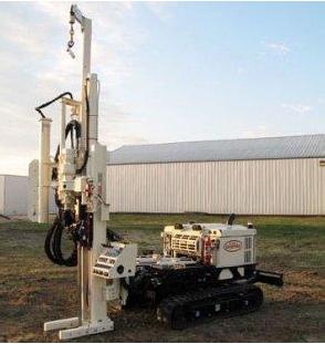
Figure 7. Percussion Hammer (Source: Geoprobe)
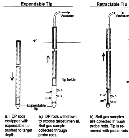
Figure 8 Direct push method (CityChlor Technical Report: Direct Push Technologies, 2013, 05)
Permanent soil-gas well installations
Usually, permanent soil-gas wells are drilling wells fitted with one screened interval. It is used to regularly monitors the soil gas at low to medium depth. Its diameter is generally from 20 mm to 80 mm and its depth is anywhere from 80 cm to several meters (depending on the water table, source, and plume locations, as well as the objectives of the study) (CityChlor, 2013).
As shown in figure 9, a solid tube assembled with a screened interval is placed in the borehole. The screened interval is located in the middle of the sand pack filled in the borehole. Then dry granular bentonite should be placed above the sand pack. From the top of dry bentonite to the surface, fill the borehole with hydrated bentonite. The function of the bentonite layer is to seal the screened interval from the surface ambient air intrusion. At last, there should be a weatherproof for the borehole, which is placed at the surface, to prevent water and ambient air intrusion. It is obtained by sufficient thickness of low permeability material, such as concrete.
This is a design of permanent wells for a simple single-depth monitoring, there are also many other more complicated designs for multi-depth soil gas monitoring.
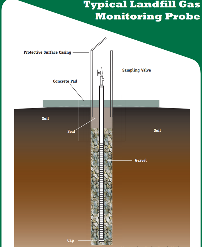
Figure 9. Permanent soil gas well (Waste Management, 2003)
Sampling Techniques
A lot of techniques can be used for soil-gas sampling.The following list brings the main techniques used in-situ:
- Reactive tubes
- Device using photo-ionization (photo ionization detector - PID)
- Measuring device detecting infrared (IR)
- Device using flame ionization (flame ionization detector - FID)
- Photo-acoustic device
- Device using gas chromatography which provides a precise concentration value for VOC (volatile organic compounds) / COHV (highly volatile organic compounds). Among the basic detectors used, FID is usually used for BTEX (benzene, toluene, ethylbenzene, and xylenes, which are main compounds of VOC) and ECD (electron capture detector) for COHV.
After sampling from the field, the gas sample is usually sent to the labrotary, and analyzed using GC-MS technique (Figure 10). GC (Gas Chromatography) is used to seperate gas mixtures into individual components using a temperature-controlled capillary column. MS (Mass Spectrometry) is used to identify the various components according to their mass spectra.

Figure 10. GC-MS Technology (Evans Analytical Group)
In the following part, three sampling methods are introduced. The first two are active sampling using pumps, and the last one is a passive sampling (sample the gas using pressure difference).
Soil-gas sampling using sample bags
Sample bags are usually used for permanent soil-gas sampling (CO2, NOx...) or ambient air sampling. Nowadays, different sorts of sample bags are available and the appropriate sampling bag should be selected depending on their properties. This method can be applied with both types of installation wells (temporary and permanent).
A sampler bag requires a pump, which is connected to the soil gas well, to pull the gas from the soil, and an inert hose (can't absorb or react with the gas components) to link the sampler bag to the pump. The sample bag size can be adjusted depending on the volume of gas necessary for the analysis (from some milliliters to several dozen liters). But The sample bag should not be filled more than 2/3 full. Then, depending on soil characteristics, soil-gas installation designs and the targeted quantification limits, sampling duration and pumping flow are determined.
After sampling, the sample bag should be stored out of sunlight, at room temperature. In the lab, gas is collected by pumping from the sample bag to an adsorbent tube, and then analyzed by GC-MS.
Soil-gas sampling using sorbent tubes
Sorbent tube is the most used sampling technique for soil-gas sampling. It can also be used for ambient air sampling. The tube is typically made of glass and contain various types of solid adsorbent materials (sorbents). The sorbents can trap and retain the compound(s) of interest in the presence of other compounds.
This method also use a pump to pull the gas from the well and let the gas go through the sorbent tube. The tube is linked to the pump by inert hose.

Figure 11. Sample bags (INERIS)
Sampling duration, pump flow, pressure, temperature should be well-mastered during the sampling event for better calculation and interpretation. Temperature and pressure may influence the volume of gas sampled. If these two parameters are monitored, recalculation can be considered to provide results under normal conditions. (CityChlor, 2013)
Once the sampling period ends, tubes should be storage in cold (< 4°C) and dark environment until their analysis. The analysis is carried out in a specific laboratory. First, trapped compounds are extracted by thermal desorption or chemical desorption and then quantified by GC-MS. Various analytical methods have been established for sorbent tubes analysis: EPA TO-17, ASTM D6196, ISO 16017, ISO 16000-6 or NIOSH 2549. Depending on the mass of the compound extracted from the sorbent tubes, the sampling flow and the sampling duration, concentration can be calculated.

Figure 12. Soil-gas sampling with sorbent tubes (INERIS)
Soil-gas sampling using Summa-Canister®
Summa-Canister® is a stainless steel container which the internal surfaces have been treated (summa process) to avoid adsorption of compounds. The use of Summa-Canister® is particularly helpful when extreme concentrations are met (both high and low concentrations). This method is different from the above two because it doesn't need a pump to sample the gas, so it's a passive sampling method. It can be used in ambient air sampling as well as soil gas.
The canister is evacuated just before it is sent to the field. The valve is opened at the beginning of the sampling event and the gas enters into the canister spontaneously (because of the difference of air pressure). This valve can be equipped with a flow controller for filling in a targeted flow rate. Filling of the canisters is controlled by the pressure gauge fitted on them.When sampling ends, the valve is closed and the whole system is sent to the analytical laboratory. Storage and transport should be carried out at room temperature. The canister is bulky and heavy, so it's difficult to transport and store it.
When returned to the laboratory, the sample should be analyzed as soon as possible. Gas is collected by pumping the gas from the canister to an adsorbent tube, then analyzed usually by GC-MS.
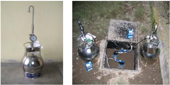
Figure 13. Summa-Canister (INERIS)
Near Surface Gas Monitoring
Near surface gas monitoring is the measurement (usually by portable instruments) of gas concentrations within a few inches of the surface of the landfill. A common method of near surface gas monitoring is the use of a portable instrument such as a flame ionization detector (FID). An FID is a scientific instrument that measures the concentration of organic species in a gas stream. The operation of the FID is based on the detection of ions formed during combustion of organic compounds in a hydrogen flame. The generation of these ions is proportional to the concentration of organic species in the sample gas stream.

Figure 14. Flame ionization detector (Matthew Klee, GC Solutions)
The sampling technician walks over the surface of the landfill in either a random method or over a pre-defined grid. The sampling technician records the instrument readings, making careful note of the geographic location of each measurement and the surface conditions, height of the probe inlet from surface, and weather conditions such as wind speed. The measurements may be recorded as parts per million by volume, percent by volume, or percent of lower explosive limit.
Recent studies has shown that using FID as the monitoring device is unreliable. Sample bag or Summa canister can also be used to get a "grab" sample of near surface gas.
Near surface gas monitoring is useful for finding cracks in landfill cover, or the proper locations of installing the soil gas wells.
Emissions Monitoring
Unlike soil gas and near surface gas monitoring, which measure the concentrations of chemicals in landfill gas, emissions monitoring measures the rates at which chemicals in landfill gases are released from landfills. Emissions sources at landfills that are most frequently monitored are the landfill surface itself and landfill gas combustion units (e.g., flares or other combustion devices).
Emissions monitoring can be used to judge the need for, or the effectiveness of, a landfill gas control system. It is also used to determine the volume of air contamination over time releasing from the landfill.
Flux Chambers
Flux chambers are used to collect the passive release of landfill gases for later analysis, either on site or in a laboratory to determine the emission rate. Surface flux chamber is set up to enclose a known surface area. It is placed directly on the surface for a known time period. It should be well-sealed against the surface. All of those chambers are designed to create good mixing and sampling conditions, minimizing the disturbance of the gas emission. A broad expanse of volatile compounds can be monitored by surface flux measurements, such as VOCs, mercury, methane, carbon dioxide, NOx, and sulfur compounds.
Static flux chamber looks like a container constructed of an inert and non-adsorbing material. It is also connected to the appropriate sampling system. The gas concentration changes with time in the chamber without intrusion of any gas outside the chamber. Contaminant flux increases over the sampling period. Discrete samples should be withdrawn at regular intervals during the whole sampling period. Static flux chamber measurement lasts from some minutes (using PID or FID) to one hour or less (using sorbent tubes for example).

Figure 15. Static-flux-chamber with PID monitoring (INERIS)
Scanning surface flux chambers are connected to an inert gas supply system and an exit fitted out with measurement points. The system gathers contaminant gas emitted from soil within the inert gas flow. Before sampling, it is necessary to reach the stabilization of the flow regime of inert carrier gas into a chamber in contact with the ground. Therefore the measured parameters (concentrations and outgoing air-flows) allow for the test to quantify the flow of emitted vapors outgoing from the chamber, and thus to deduce the flow released through the concrete slab or the ground.The surface flux chamber needs a longer period of equilibration due to its size and the gas injection. Flux measurement lasts around three or four hours.

Figure 16. Scanning flux chamber with PID monitoring (INERIS)
Spectroscopic Sampling Techniques
Surface emissions are also being measured by Fourier-transformed infrared-red (FTIR) or ultra-violet spectroscopy (UVS) sampling techniques. These techniques can detect and identify contaminants in the air along a straight line (e.g., the boundary of a landfill or across the landfill surface). UVS is typically set up for specific compounds (usually inorganic gases), but FTIR can be used for multiple compounds (usually organic gases). The spectroanalysis can identify specific compounds and concentrations in the space between the source and the receptor. (Agency for Toxic Substances and Disease Registry, 2001)
The website of Emission Measurement Center (EMC) of EPA compiles a long list of the test methods available for emission measurement.
Ambient Air and Indoor Air Monitoring
Ambient air monitoring measures levels of contamination in outdoor air, or in the air that people breathe. The levels of pollution measured in the ambient air reflect the combined influences of many different nearby sources, and even some distant ones.Indoor air monitoring is the measurement of air concentrations of contaminants in indoor or enclosed locations. Sampling locations for indoor air monitoring efforts include, but are not limited to, basements of buildings (residential, commercial, and industrial), living spaces in homes, and office spaces near landfills. (ATSDR, 2001)
Ambient air monitoring and indoor air monitoring data can provide a better characterization of gases in the breathing zone. EPA has approved several different types of sampling and analytical methods for common air pollutants, which can be found on Ambient Monitoring Technology Information Center of EPA website.
Landfill Gas Monitoring Regulations
The United States’ first attempt at regulation of air pollution was passed in 1955, called the Air Pollution Control Act. It was passed more on the basis of freeing up funds for federal government research of air pollution. However it was not until 1970 that the federal government passed the clean air act that included Emissions Guidelines (EG) for regulation of existing landfills and New Source Performance Guidelines (NSPS) for new landfills. The federal government published minimum requirements but provided the states authority to implement stronger regulations. The EG apply to any landfill that was constructed before 1991 and has accepted waste since 1987. In the following sections, the minimum federal standards will be outlined. These standards should be used in determining necessity of using monitoring methods highlighted above. Sections referring to the control devices is literature not further discussed in this paper, but important in the design of safe landfills, a main purpose of the report.
Characteristics of Landfills Requiring Monitoring
A landfill is required to be regulated based on the Non-Methane Organic Compund (NMOC) emission rate. It is very difficult to quantify the Landfill Gas (LFG), so for regulation standards, NMOC output levels are representative of LFG outputs. If a landfill has an NMOC emission rate of 50 Mg/year or more, the landfill operator is required to install a gas collection and control device system to regulate hazardous emissions.
If the landfill has a NMOC less than 50 Mg/year, the landfill owner must provide a yearly report of NMOC levels until the landfill is either no longer accepting waste, or levels rise above 50 Mg/year in which case a collection system must be installed as discussed above. The EPA requires periodical monitoring of NMOC emissions as they will fluctuate over time. (EPA, 1999)
Required Technology
Gas collection technologies are required by the EPA in active areas of the landfill. Active areas are those where the waste is producing gasses and are exposed to the environment. This is defined as locations in the landfill where either no more waste is being deposited in the cell, or where the first refuses are 5 years or older. The latter of these, called active areas, must be controlled even though waste is still being added to the area. Closed areas must have gas collection systems if the oldest waste is 2 years or older.
Federal regulations allow for a variety of gas collection technologies to be used. Because of the wide variety of site specific characteristics, many alternative systems may be utilized; however the most common collection systems are active and passive systems. Landfills are required to submit a Collection and Control System Design Plan prepared by a professional engineer that will be submitted to a regulatory agency for authorization to move forward with plans. For an active system, the plan must be designed to satisfy the following:
- Handle the maximum expected gas flow rate over the expected lifespan of collection system equipment,
- Collect gas from each area or cell in which solid waste has been placed for 5 years if the cell is active and 2 years if it is closed or at final grade,
- Collect gas at a sufficient extraction rate (A sufficient extraction rate is a rate adequate to maintain a negative pressure at all wellheads in the collection system without causing air infiltration.), and
- Minimize off-site migration of subsurface gas.
Passive systems must satisfy 1), 2), and 4) as well as have liners at the boundaries of the gas collection area. Both active and passive systems must direct the collected gas to a control device. (EPA, 1999)
Gas Collection System Requirements
For a landfill gas collection to be working most effectively, the system must be operating at a sufficient gas removal rate. The EPA provides some broad guidelines for this sufficiency. Each wellhead in the collection system must be sustained in order to direct the gas into the collection system rather than letting it escape. However, if the rate of gas extraction is too high, air from outside of the system will leak in, spiking the densities of some gasses. An insufficient collection rate may lead to LFG leaking out of the system and into the environment around. If the methane level at the ground surface of the landfill is greater than 500 parts per million, the collection rate is deemed inadequate.
Collection system parameters must also be periodically monitored, including pressure, nitrogen concentration, oxygen concentration, temperature, surface methane concentration. If these results are outside of an acceptable value, the collection system will need to be modified or upgraded, depending on the situation. Whatever design variances to the system parameters must presented to the State agency with justification, which will either to be approved or disapproved.
LFG is routed through the collection system to a control device. This control device, which is selected for the particular system must be running at all times besides start and stop times, and when it is malfunctioning. As long as all times when the collection system is inoperable for less than 5 days, it is allowable. If the period of malfunctioning is longer than 5 days, the collection system must be sealed and the valves closed to contain the dangerous gasses from leaking into the atmosphere. (EPA, 1999)
Gas Control Device Requirements
The EPA’s suggestion for a best designed technology (BDT) for controlling the emissions is a device capable of reducing NMOC emissions by 98 weight-percent or reducing emissions to 20 parts per million by volume dry (ppmvd) as hexane. Devices deemed acceptable include open flares and enclosed combustion devices.
For flares, measurement of reduction percentage or gas concentration of the outlet is not feasible, so it is difficult to numerically evaluate emission performance. Instead, flares are approved or denied based on how they meet specifications provided by the EPA that are assumed to have 98% control. Therefore, a performance test is not required. Enclosed combustion devices are much more feasible to complete performance tests on. These performance tests must be in accordance with EPA methods.
The control device is required to be operating at all times outside of start and stop sequences, as well as malfunctions. Like the collection system, there is a 1 hour grace period for how long it is acceptable to be out of commission. If the control device is out of commission for longer than 1 hour, the collection system must be shut down and all atmospheric valves must be closed. (EPA, 1999)
Compliance Schedule
Figure 17 provides a sample compliance schedule based on a promulgation of a landfill on March 12, 1996.

Figure 17. Compliance Schedule (EPA, 1999)
Gas Collection and Control Device Removal Guidelines
Gas collection and control systems can be capped or removed when all of the conditions listed below are satisfied (EPA, 1999):
- The landfill is closed,
- The landfill owner or operator notifies the implementing agency by submitting a Landfill Closure Report,
- The gas collection and control system has been operating continuously for at least 15 years, and
- The landfill NMOC emission rate has been calculated to be less than 50 Mg/yr on three successive test dates. The test dates should be no closer than 90 days apart and no farther than 180 days apart
References
- Atlanta Journal-Constitution. (1999) Mysterious gas blast closes park. February 9, 1999.
- A. Tre Âgoure Ás, (1999) “Comparison of seven methods for measuring methane flux at a municipal solid waste landfill site”, Waste Management & Research, ISSN 0734-242X.
- ATSDR (Agency for Toxic Substances and Disease Registry). (2001) “Landfill Gas Primer: an overview for environmental health professionals.”
- Bart Eklund, Eric P. Anderson, Barry L. Walker, and Don B. Burrows. (1998) “Characterization of Landfill Gas Composition at the Fresh Kills Municipal Solid-Waste Landfill”, Environ. Sci. Technol. 32, 2233-2237.
- Charlotte Observer. (1994) “Woman severely burned playing soccer”. November 7, 1994.
- CityChlor (2013) “Soil-Gas Monitoring: Soil Gas Well Designs and Soil-Gas Sampling Techniques”, DRC-13-114341-03542A.
- Environment Agency. (2010) “Guidance on monitoring landfill gas surface emissions”, LFTGN07 v2.
- Gazasia. http://gazasia.com/biogas-source/landfill-sites-2/
- Gino Yekta. (2014) “Basic Landfill Gas Monitoring Training.”
- G. Tchobanoglous, H. Theisen and S. Vigil. (1993) "Integrated Solid Waste Management, Engineering Principles and Management Issues," McGraw-Hill, New York.
- Hans Oonk. (2010) “Literature Review: Methane from Landfills.”
- Hari D. Sharma and Krishna R. Reddy. (2004) “Geoenvironmental Engineering: Site remediation, waste containment, and emerging waste management technologies,” Wiley.
- H. Kamalan, M. Sabour and N. Shariatmadari. (2011) “A Review on Available Landfill Gas Models,” Journal of environmental science and technology 4 (2): 79-92.
- Matthew Klee, “GC Solutions #11: The Flame Ionization Detector.”
- Tchobanoglous G, Theisen H, and Vigil S. (1993) “Integrated Solid Waste Management, Engineering Principles and Management Issues”. New York: McGraw-Hill.
- United States Environmental Protection Agency (2005) “Landfill Gas Emissions Model (LandGEM) Version 3.02 User’s Guide”, EPA-600/R-05/047 May 2005.
- U.S. Army Corps of Engineers. (1995) “Landfill Off-Gas Collection and Treatment System”, ETL 1110-1-160, U.S. Department of the Army, Washington, DC.
- U.S. Army Corps of Engineers. (1984) “Landfill gas control at military installations”, Prepared by R.A. Shafer. Publication Number CERL-TR-N-173. January 1984.
- U.S. Environmental Protection Agency Reports. (2012) “International Best Practices Guide for Landfill Gas Energy Project.”
- U.S. Environmental Protection Agency Reports. (2015a) “Inventory of U.S. Greenhouse Gas Emissions and Sinks”: 1990-2013, 430-R-15-004.
- U.S. Environmental Protection Agency Reports. (2015b) “LFG Energy Project Development Handbook.”
- U.S. Environmental Protection Agency Reports. (1999) "Summary of the Requirements for the New Source Performance Standards and Emission Guidelines for Municipal Solid Waste Landfills." 1 Feb. 1999. Web. 18 Nov. 2015.
 Dowon Park
  Tianqi Zhao
  Zachary Goulson
 Industry News


Events

12th International Symposium on Field Monitoring in Geomechanics 2026

DFI 50th Anniversary Conference on Deep Foundations

9th International Symposium for Geotechnical Safety and Risk

5th International Symposium on Frontiers in Offshore Geotechnics (ISFOG)

Pan Mediterranean Geotechnical Engineering Conference

The Third Vietnam Symposium on Advances in Offshore Engineering

4th Asia-Pacific Conference on Physical Modelling in Geotechnics (ACPMG 2024)

The 2nd GeoMandu: Geotechnics for Sustainable Infrastructures

5th International Conference on Transportation Geotechnics


2 COMMENTS
Jason D. x*
Dec, 12, 2015 Thank you for a comprehensive report. I am curious if you could elaborate on the various models used for emissions. What are the advantages and disadvantages? Which ones are used the most outside the US? Dowon Park
Dec, 17, 2015 Thank you for your comment. In the project report, list of various models, their specification, general comparison are presented briefly because the emphasis on the project is landfill gas monitoring system than landfill gas emission models. In addition to this, I organized primary landfill gas models like LandGEM, IPCC and country-specific models in terms of advantages and disadvantages.The U.S. EPA’s Landfill Gas Emissions Model (LandGEM) was designed for estimating emissions of various landfill gas components from U.S. landfills. It uses the first-order exponential equation to estimate methane generation. The main variables in the first order decay equation are the methane generation rate constant (k), and the potential methane generation capacity (L0).
The default k and L0 values may be appropriate for modeling LFG generation from U.S. landfills that are characterized by U.S. landfill data, but they often are not appropriate when estimate landfill sites that may show different climate conditions and waste composition, which cause dramatic difference of LFG generation.
Example. 1: LandGEM Limitations for Moisture Conditions, (US EPA, 2012)
The range of default k values in LandGEM for non-bioreactor (arid and conventional) landfills is limited to 0.02 for sites that experience less than 25 inches (635 millimeters [mm]) of precipitation per year and 0.04 or 0.05 for sites that experience higher rainfall amounts. This range of values may reflect the typical range of moisture conditions found in most landfills in the U.S., but most tropical countries have regions where rainfall commonly exceeds 2,000 mm/year and can exceed 4,000 mm/year. LandGEM does not provide any guidance on appropriate k values for such rainy climates.
Also, a high percentage of food waste contribute to different pattern of waste decomposition rate over time. Because organic waste decays more rapidly than other organic materials, it also is depleted more rapidly once waste disposal stops.
Another landfill gas emissions model is the Intergovernmental Panel on Climate Change (IPCC) Model which is designed for worldwide applications. Like LandGEM, the IPCC Model uses a first-order decay equation that applies annual waste disposal rates and a waste decay rate variable (k value). However, the first-order calculations do not include the LandGEM variable L0, instead include other variables such as DOC, DOCf, MCF which are related to L0 when combined together.
Since the IPCC model includes features that make it appropriate for modeling non-U.S. landfill sites, the IPCC Model is currently the best available tool for estimating LFG generation in most outside the US. However, it is not precise in its accounting for particular conditions of each countries because it is a global model.
Example. 2: IPCC Limitations for precipitation, (US EPA, 2012)
The 1,000 mm/year precipitation threshold for separating tropical climates into dry vs. wet categories is better than the LandGEM threshold of 635 mm/year (25 inches/year) but is likely too coarse to account for the effects of precipitation across the wide range of values encountered. For example, most areas in Colombia experience more than 1,000 mm/year of precipitation and many areas get more than 2,000 mm/year. Landfills in these areas would be treated the same (identical k values) in the IPCC Model, which implies that there are no noticeable effects from increasing precipitation above 1,000 mm/year.
Besides LandGEM and IPCC model, there are many country-specific models that apply the structure of either LandGEM or the IPCC Model, but combine it with detailed information from each country to produce models that more realistically reflect local conditions which affect landfill gas generation. Below link indicates country-specific models, such as Central America, China, Colombia, Ecuador, Mexico, Philippines, Thailand, Ukraine LFG models. Those models has been developed based on the research of the regional climates and define k and L0 variables which are appropriate for the climate of the landfills.
http://www3.epa.gov/lmop/publications-tools/index.html#three
Thank you again for your valuable comment.
Edit Comment